Lesson 5Using Dot Plots to Answer Statistical Questions
Let's use dot plots to describe distributions and answer questions.
Learning Targets:
- I can use a dot plot to represent the distribution of a data set and answer questions about the real-world situation.
- I can use center and spread to describe data sets, including what is typical in a data set.
5.1 Packs on Backs
This dot plot shows the weights of backpacks, in kilograms, of 50 sixth-grade students at a school in New Zealand.

- The dot plot shows several dots at 0 kilograms. What could a value of 0 mean in this context?
-
Clare and Tyler studied the dot plot.
- Clare said, “I think we can use 3 kilograms to describe a typical backpack weight of the group because it represents 20%—or the largest portion—of the data.”
-
Tyler disagreed and said, “I think 3 kilograms is too low to describe a typical weight. Half of the dots are for backpacks that are heavier than 3 kilograms, so I would use a larger value.”
Do you agree with either of them? Explain your reasoning.
5.2 On the Phone
Twenty-five sixth-grade students were asked to estimate how many hours a week they spend talking on the phone. This dot plot represents their reported number of hours of phone usage per week.

-
- How many of the students reported not talking on the phone during the week? Explain how you know.
- What percentage of the students reported not talking on the phone?
-
- What is the largest number of hours a student spent talking on the phone per week?
- What percentage of the group reported talking on the phone for this amount of time?
-
- How many hours would you say that these students typically spend talking on the phone?
- How many minutes per day would that be?
-
- How would you describe the spread of the data? Would you consider these students’ amounts of time on the phone to be alike or different? Explain your reasoning.
- Here is the dot plot from an earlier activity. It shows the number of hours per week the same group of 25 sixth-grade students reported spending on homework.

Overall, are these students more alike in the amount of time they spend talking on the phone or in the amount of time they spend on homework? Explain your reasoning.
- Suppose someone claimed that these sixth-grade students spend too much time on the phone. Do you agree? Use your analysis of the dot plot to support your answer.
5.3 Clickety-Clackety
- A keyboarding teacher wondered: “Do typing speeds of students improve after taking a keyboarding course?” Explain why her question is a statistical question.
- The teacher recorded the number of words that her students could type per minute at the beginning of a course and again at the end. The two dot plots show the two data sets.

Based on the dot plots, do you agree with each of the following statements about this group of students? Be prepared to explain your reasoning.
-
Overall, the students’ typing speed did not improve. They typed at the same speed at the end of the course as they did at the beginning.
-
20 words per minute is a good estimate for how fast, in general, the students typed at the beginning of the course.
-
20 words per minute is a good description of the center of the data set at the end of the course.
-
There was more variability in the typing speeds at the beginning of the course than at the end, so the students’ typing speeds were more alike at the end.
-
-
Overall, how fast would you say that the students typed after completing the course? What would you consider the center of the end-of-course data?
Are you ready for more?
Use one of these suggestions (or make up your own). Research to create a dot plot with at least 10 values. Then, describe the center and spread of the distribution.
- Points scored by your favorite sports team in its last 10 games
- Length of your 10 favorite movies (in minutes)
- Ages of your favorite 10 celebrities
Lesson 5 Summary
One way to describe what is typical or characteristic for a data set is by looking at the center and spread of its distribution.
Let’s compare the distribution of cat weights and dog weights shown on these dot plots.


The collection of points for the cat data is further to the left on the number line than the dog data. Based on the dot plots, we may describe the center of the distribution for cat weights to be between 4 and 5 kilograms and the center for dog weights to be between 7 and 8 kilograms.
We often say that values at or near the center of a distribution are typical for that group. This means that a weight of 4–5 kilograms is typical for a cat in the data set, and weight of 7–8 kilograms is typical for a dog.
We also see that the dog weights are more spread out than the cat weights. The difference between the heaviest and lightest cats is only 4 kilograms, but the difference between the heaviest and lightest dogs is 6 kilograms.
A distribution with greater spread tells us that the data have greater variability. In this case, we could say that the cats are more similar in their weights than the dogs.
In future lessons, we will discuss how to measure the center and spread of a distribution.
Glossary Terms
The center of a set of numerical data is a value in the middle of the distribution. It represents a typical value for the data set.
For example, the center of this distribution of cat weights is between 4.5 and 5 kilograms.
The spread of a set of numerical data tells how far apart the values are.
For example, the dot plots show that the travel times for students in South Africa are more spread out than for New Zealand.

Lesson 5 Practice Problems
Three sets of data about ten sixth-grade students were used to make three dot plots. The person who made these dot plots forgot to label them. Match each dot plot with the appropriate label.
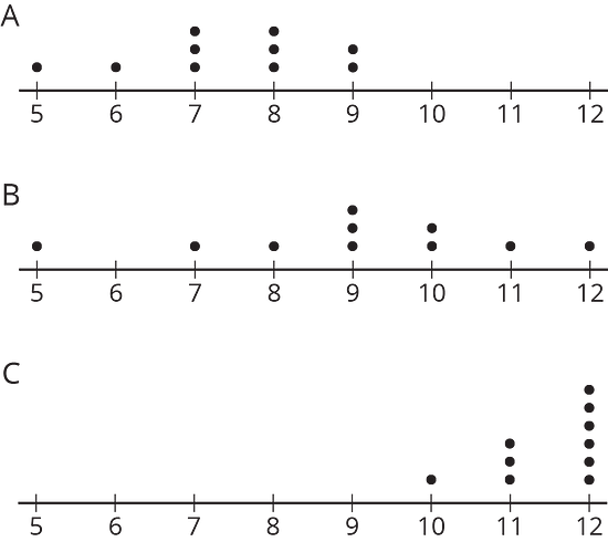
- Ages in years
- Numbers of hours of sleep on nights before school days
- Numbers of hours of sleep on nights before non-school days
The dot plots show the time it takes to get to school for ten sixth-grade students from the United States, Canada, Australia, New Zealand, and South Africa.

- List the countries in order of typical travel times, from shortest to longest.
- List the countries in order of variability in travel times, from the least variability to the greatest.
Twenty-five students were asked to rate—on a scale of 0 to 10—how important it is to reduce pollution. A rating of 0 means “not at all important” and a rating of 10 means “very important.” Here is a dot plot of their responses.

Explain why a rating of 6 is not a good description of the center of this data set.
Tyler wants to buy some cherries at the farmer’s market. He has $10 and cherries cost $4 per pound.
- If is the number of pounds of cherries that Tyler can buy, write one or more inequalities or equations describing .
- Can 2 be a value of ? Can 3 be a value of ? What about -1? Explain your reasoning.
- If is the amount of money, in dollars, Tyler can spend, write one or more inequalities or equations describing .
- Can 8 be a value of ? Can 2 be a value of ? What about 10.5? Explain your reasoning.