Here are the weights, in kilograms, of 30 dogs.
| 10 |
11 |
12 |
12 |
13 |
15 |
16 |
16 |
17 |
18 |
| 18 |
19 |
20 |
20 |
20 |
21 |
22 |
22 |
22 |
23 |
| 24 |
24 |
26 |
26 |
28 |
30 |
32 |
32 |
34 |
34 |
Before we draw a histogram, let’s consider a couple of questions.
-
What are the smallest and largest values in our data set? This gives us an idea of the distance on the number line that our histogram will cover. In this case, the minimum is 10 and the maximum is 34, so our number line needs to extend from 10 to 35 at the very least.
(Remember the convention we use to mark off the number line for a histogram: we include the left boundary of a bar but exclude the right boundary. If 34 is the right boundary of the last bar, it won't be included in that bar, so the number line needs to go a little greater than the maximum value.)
-
What group size or bin size seems reasonable here? We could organize the weights into bins of 2 kilograms (10, 12, 14, . . .), 5 kilograms, (10, 15, 20, 25, . . .), 10 kilograms (10, 20, 30, . . .), or any other size. The smaller the bins, the more bars we will have, and vice versa.
Let’s use bins of 5 kilograms for the dog weights. The boundaries of our bins will be: 10, 15, 20, 25, 30, 35. We stop at 35 because it is greater than the maximum.
Next, we find the frequency for the values in each group. It is helpful to organize the values in a table.
| |
weights in kilograms |
frequency |
| row 1 |
10 to less than 15 |
5 |
| row 2 |
15 to less than 20 |
7 |
| row 3 |
20 to less than 25 |
10 |
| row 4 |
25 to less than 30 |
3 |
| row 5 |
30 to less than 35 |
5 |
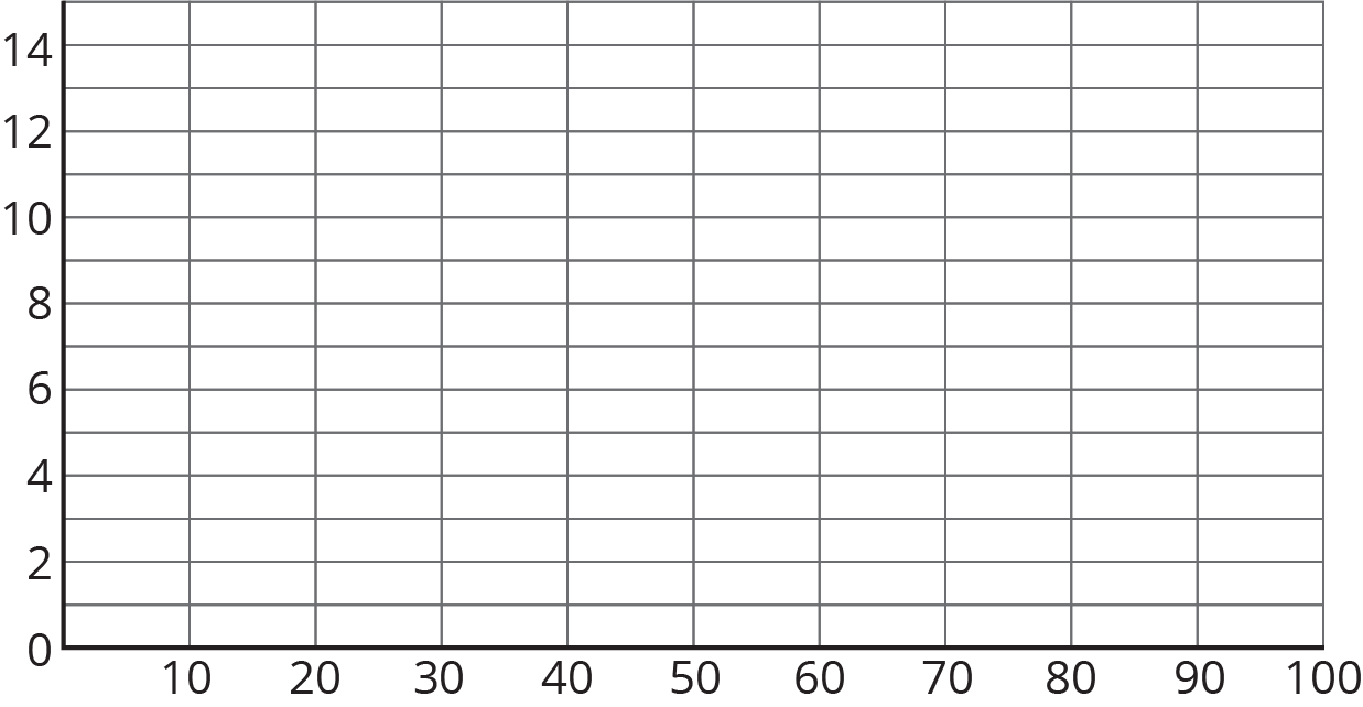
Now we can draw the histogram.

The histogram allows us to learn more about the dog weight distribution and describe its center and spread.


